Quick Start: Browsing an Horizontal Dilatometer file¶

This Demo will guide you through the data analysis of Horizontal Dilatometer (horizontal) output files.

In order to follow the tutorial you should:

Download and Install Misura™ (see Installation).

Get the sample file Horizontal Dilatometer Sample File 1.h5 and save it to a known location (eg: your Desktop)

Opening the output file¶

Run browser.exe application from the folder where you extracted Misura™, or run the link you created on your desktop.
In the Recent data sources window, under the first column Recent files, click on Add button.
Browse to the location where you downloaded Horizontal Dilatometer Sample File 1.h5, select and open it.
The loading process will start. If the file is considerably big (several GB) or located on network or slow storage drive, it may take several seconds to open.
The file is displayed on a new tab, on the right of the Databases tab.

The test file tab is divided in three areas:

A menu bar in the upper part of the window
A right area called Test Configuration. It is divided in at least 4 vertical tabs: Measure, Thermal Cycle, Sample0 and Results.
A central area displaying movable and resizable sub-windows, where you see the Data Plot window.

Test Configuration and Data¶

The most relevant configuration options used for the test run and output results are displayed in the right Test Configuration area.

Measure overview¶

The first Measure tab contains the list of options regarding the test run.

Detect the following:

Name: Name of the test run, set by the operator anytime before the end of the test.
Operator: the login name used by the operator who started the test.
Type: The type of the test (usually Standard or Calibration).
Elapsed time: the total duration of the test.

Thermal cycle¶

This tab contains a table with points defining the thermal cycle and a graph with a cartesian representation.

The graph displays two curves: the red line is the setpoint temperature; the blue line is the heating rate.

If you cannot see the axes and their labels, enlarge the application window and the Test Configuration area.

Sample data¶

Most relevant data in the Sample0 tab are:

Name: if set, the name the operator gave to this specific sample. It is mainly useful for multi-sample measurement.
Initial sample dimension: the operator must set this value to the initial sample length, measured with another instrument (eg: a digital micrometer).
Record frames/profiles: did the operator required full frames and (x,y) sample profiles to be recorded onto the output file? They are usually turned off.

You can ignore Border angle, Motion start, Total displacement, Cumulative error options an all their nested options, as they are only useful during live acquisition.

Results¶

The Results tab displays the Navigator tree component. It is the tree of recorded datasets (curves), organized by groups. Each group represents a part of the instrument or of the measurement.

For example:

/horizontal element represents the Horizontal Dilatometer instrument itself. It generates no datasets, but contains one sample (sample0).
/kiln element represents the furnace, and contains datasets regarding temperature control (T, temperature; S, setpoint; P, power; etc).

We will see it in detail in next sections, as it is the most powerful and versatile component of the interface.

Interacting with the Data Plot¶

The Misura™ Navigator tree is the gate to the most important actions you can perform on the data plot.

In order to plot one more dataset (for example the temperature setpoint):

Right-click on the dataset you wish to plot on the Navigator tree (/kiln/S).
Select the Plot action from the context menu.

The same apply for removing a dataset and all its related objects from the plot. The Plot action will be checked if the curve is visible, unchecked if not visibile.

The setpoint curve plot is now referred to its own axis labelled S (°C). To better compare temperature and setpoint, it is useful to refer the setpoint plot to the temperature axis:

Right-click on the setpoint curve on the Data Plot window. Select Properties from the context menu.
A new dialog window opens, listing all the properties of the plotted curve. Search for the bold Y axis entry.
Change Y axis from ax:S to ax:T. The curve will be immediately referred to the T (°C) axis.

The S (°C) axis loses its scale (it’s now from 0 to 1). It’s no longer useful, so you can hide it:

Right-click on the S (°C) axis, select Properties.
The first entry is Hide. Check the checkbox. The axis disappears.

You can freely move any axis by clicking on it and dragging.

Viewing dilatation as Percentile¶

The /horizontal/sample0/d dataset represents dilatation. It is recorded in microns, but is frequently useful to analyze it as a percentile of the total initial length of the sample. The initial length was measured with a manual digital micrometer, and set before starting the test.

Follow these steps to convert the curve to percentile:

Locate the d (/horizontal/sample0/d) element in the Navigator tree under Results tab.
Right-click and select Percentile.
A dialog will appear. Click Apply.
A new temporary label in the dialog confirms the dataset was created (Done). Click Close.
If the curve is currently plotted, you immediately view the effect in the graph.

It may happen that the operator forget to measure the sample, or inserts a wrong initial dimension. If the thermal treatment modify the structure of your material, the test must be repeated. In case you are able to recover the correct intial dimension, or you are confident that you can measure it after the test run, you can change its value.

Locate the d element in the Navigator tree.
Right-click and select Set Initial Dimension.
Insert the correct value in Initial dimension value.
De-select OR, automatic calculation based on first points checkbox.
Click Apply then Close.

If the curve is currently plotted in percentile, you will se the axis scale changing accordingly to the new initial dimension set.

Evaluating the Coefficient of Expansion¶

The coefficient of expansion is calculated from the d dataset, the initial dimension and the temperature. To create the coefficient curve:

Locate the d element in the Navigator tree.
Right-click and select Linear Coefficient.
Click Apply and Close.
The Navigator tree is updated. The d element now has a child: Coefficient(T,d). This is the coefficient of expansion.
Plot the coefficient dataset using its context menu.

The curve will be referred to a new axis Coeff(50). The number 50 in the label means the coefficient was calculated starting from 50°C. The scale of the axis will be around 10^-6 - 10^-5. You can rescale the axis to a more comfortable multiplier:

Right-click on the Coeff(50) axis. Select Properties action.
Locate the Scale entry and set it to 1e6.

Now the scale of the axis should go from 2.5 to 12.5, where the multiplier is 10^-6.

Calibrating with a known standard¶

By comparing the measured expansion curve of a standard material with theoretical values, it is possible to calculate a calibration factor which can then be applied directly during the measurement. The calibration factor will be multiplied by the observed expansion, acting as a slope correction on the whole expansion curve.

If the factor is less than one, it means the measured curve of the standard material was higher than the theoretical, so all measurements will be reduced by that number. In case the factor is greater than one, it means the measurement was lower: all subsequent measurements will be increased accordingly.

To execute the calibration tool, open the test in the Browser or Graphics, then:

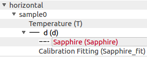
Locate the d element in the Navigator tree.
Right-click and select Calibration.
Select the Calibration standard, start/end temperature and display options.
Click Apply and Close.

When launched through this sequence, the calibration plugin dialog will show pre-filled fields for Expansion dataset and Temperature dataset:

Other options include:

Calibration Standard chooser contains a list of materials having certified expansion curves.
First temperature margin determines the temperature interval to discard from the start of the test. When the test starts, thermal control might induce imperfections in the heating rate, due to furnace inertia. This options allows to ignore the initial part of the curve.
Last temperature margin allows to discard a temperature interval at the end of the test.
Draw calibration label will create a text label on the currently selected plot page, and output the calibration factor and standard deviation.
Add calibration datasets will add the theoretical expansion values and a polynomial fit of the measured values to two child datasets. Those curves can later be plotted.
Start index allows to skip initial points by index (second) - alternative to First temperature margin

Example navigator tree after the creation of calibration datasets:

Example calibration plot with calibration label and plotted standard:

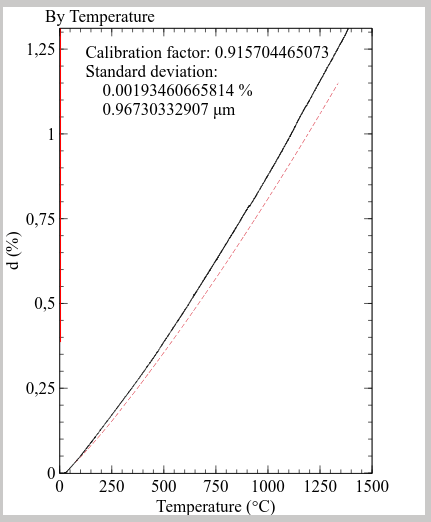
The calibration factor can then be copied from the label and configured in the Settings ‣ Instrument panel under ref:live_acquisition.

This procedure works both on native Misura™ tests and on imported Misura3 tests.