Quick Start: Browsing a Microscope file
This Demo will guide you through the data analysis of Heating Microscope (hsm) output files.
In order to follow the tutorial you should:
- Download and Install Misura™ (see Installation).
- Get the sample file Microscope Sample File 1.h5 and save it to a known location (eg: your Desktop)
Opening the output file
- Run
browser.exeapplication from the folder where you extracted Misura™, or run the link you created on your desktop. - In the Recent data sources window, under the first column Recent files, click on Add button.
- Browse to the location where you downloaded Microscope Sample File 1.h5, select and open it.
- The loading process will start. If the file is considerably big (several GB) or located on network or slow storage drive, it may take several seconds to open.
- The file is displayed on a new tab, on the right of the Databases tab.
The test file tab is divided in three areas:
- A menu bar in the upper part of the window
- A right area called Test Configuration. It is divided in at least 4 vertical tabs: Measure, Thermal Cycle, Sample0 and Results.
- A central area displaying movable and resizable sub-windows, where you see the Data Plot window.
Test Configuration and Data
The most relevant configuration options used for the test run and output results are displayed in the right Test Configuration area.
Measure overview
The first Measure tab contains the list of options regarding the test run.
Detect the following:
- Name: Name of the test run, set by the operator anytime before the end of the test.
- Operator: the login name used by the operator who started the test.
- Elapsed time: the total duration of the test.
Measurement Units
Elapsed time is expressed, by default, in seconds unit. This might be difficult to read. You can change the measurement unit of any value listed in Misura™ options panels by following this steps:
- Right click on the Elapsed time text label. A menu will popup.
- Select the Units sub-menu.
- Change to your preferred unit. E.g.: minute.
- You can roll-back to second by repeating the procedure.
Hint
If the Units sub-menu is not shown, it means the option does not have a specific measurement unit set, so it cannot be converted.
Metadata
The following values (after Elapsed time) are called Metadata or, more specifically, characteristic points. For example:
- End of the test: it contains time and temperature values recorded when the test ended.
- Maximum temperature: time and temperature of the point when maximum temperature was reached.
- Maximum Heating Rate: time and temperature of the point when the maximum punctual heating rate was reached in the measured temperature profile.
By clicking on the last one, a new window will open displaying again time and temperature, plus a Value number. In the case of Maximum Heating Rate, this number is the actual heating rate (°C/s) measured in that point.
Hint
At the end of each Metadata row there is a + sign button. It means there are nested options under the visible one. By clicking on it, access to another option, viewed as a Edit button. By clicking on it, you open an editor where you can read the logic used to calculate the parent Metadata point.
General measurement Metadata are usually short and simple to understand.
Thermal cycle
This tab contains a table with points defining the thermal cycle and a graph with a cartesian representation.
The graph displays two curves: the red line is the setpoint temperature; the blue line is the heating rate.
If you cannot see the axes and their labels, enlarge the application window and the Test Configuration area.
Sample data
Most relevant data in the Sample0 tab are:
- Name: if set, the name the operator gave to this specific sample. It is mainly useful for multi-sample measurement.
- Initial sample dimension: the operator can optionally set this value if he measured the initial sample height with other instruments (eg: a digital micrometer).
- Record frames/profiles: did the operator required full frames and (x,y) sample profiles to be recorded onto the output file? In the case of Microscope Sample File 1.h5, only profiles were required, in order to keep the file smaller.
You can ignore Height, Perimeter, Volume options an all their nested options, as they are only useful during live acquisition.
Of paramount importance are the five Characteristic Points, expressed as Metadata options. They are defined and identified according to the highly reliable Misura™ standard.
- Sintering
- Softening
- Sphere
- HalfSphere
- Melting
Re-evaluating Standards
As the logic by which characteristic points are identified is accessible from the Misura™ Browser, you can also change it and see the effect on the identified points. This process is called Standard Re-Evaluation, as this logic is usually codified in an international standard depending on your material.
As an example, we will affect the Sintering point.
- Take not of the current value of Temp:/Time: label (611.0, 1805.0).
- Click on the [+] button right to the Temp:/Time: label.
- Change the Height shrinking for Sintering from 95 to 90.
- Locate the Measure menu on the upper-left menu bar. Click on the Re-evaluate standards action.
- Move your mouse on the Sintering label. It will update to a different Temp:/Time: point (621.0, 1836.3).
You required a higher shrinking in order to detect the Sintering point, so the point is now identified 10°C above its original value.
Results
The Results tab displays the Misura™ Navigator tree component. It is the tree of recorded datasets (curves), organized by groups. Each group represents a parts of the instrument or of the measurement.
For example:
- hsm represents the Microscope instruments itself. It generates no datasets, but contains one sample (sample0). If we have a multi-sample test, it will contain one sub group for each sample.
- kiln represents the furnace, and contains datasets regarding temperature control (T, temperature; S, setpoint; P, power; etc).
We will see it in detail in next sections, as it is the most powerful and versatile component of the interface.
Visual shape assessment
To understand the behaviour of your material with time and temperature change, you will use three main tools:
- The Story Board, where you can see the shape of your sample at the desired time in the test.
- The Navigator tree in Results tab contained in the Test Configuration area, where you can see the exact value of each calculated output.
- The Data Plot, where you can evaluate the behaviour and rate of change of each plotted datasets.
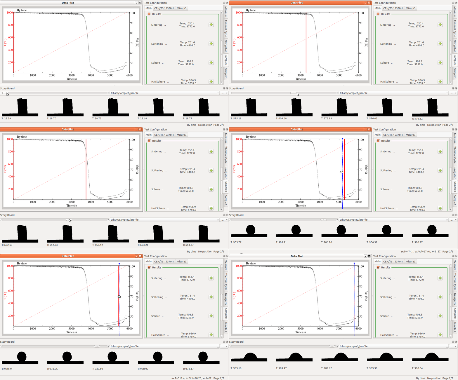
These tools are all synchronized at the same time in the test. When you move the horizontal slider in the Snapshot area, the images are updated to reflect the state of the sample at the selected point. At the same time, a vertical red bar updates its position on the Data Plot, and Navigator tree changes in order to display the current values at that point.
The point selection can happen either:
by moving the Snapshot horizontal slider
by clicking on the red bar in Data Plot and dragging in a new position
by dragging the label showing the characteristic point value (eg: Sintering) and dropping it on the Story Board. The Story Board and the plot will sync to the requested time.
The Story Board area also displays the temperature value associated to each image. You can add more values by dragging them from the Navigator tree and dropping them in the Story Board area. To remove unnecessary values, right click on them and de-select from the Labels popup sub-menu.
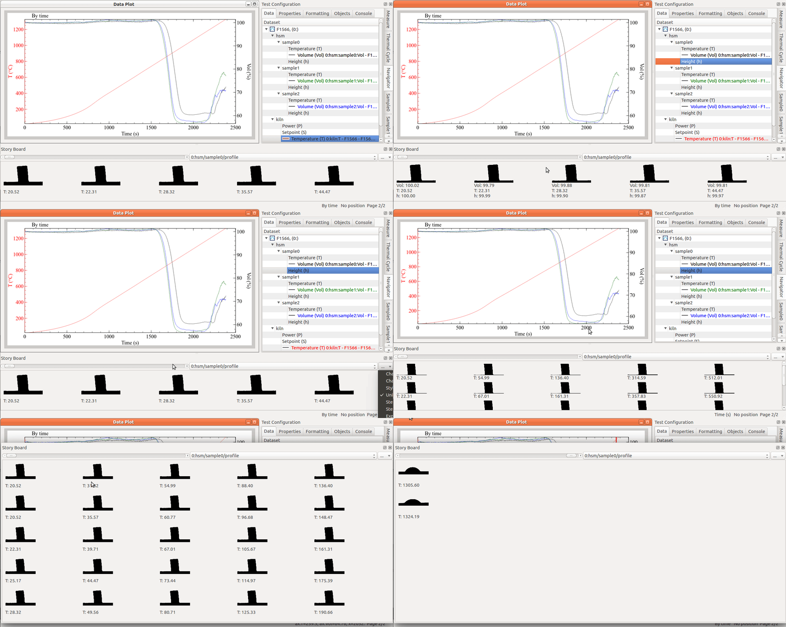
The legnth, number of rows and stepping of the storyboard can be changed from the context menu that can be called by right-clicking on the horizontal scroll bar or by clicking on the (…) button on the right of the current sample name.
Characteristic points on the Data Plot
Characteritics points are connected to the behaviour of dimensional shape measurements as a function of temperature and time. It is thus interesting to evaluate their position on the plot.
The command to add characteristic points is located in the Navigator tree context menu, accessible by right clicking on tree elements.
As Navigator tree elements represent different parts of the measurement instrument (datasets, samples, instruments, devices, etc), the menu which pops-up depends on the kind of element.
- Click on a blank area inside x,y ranges of Data Plot graph. A blue dashed line will appear over the plot area, meaning you correctly selected the graph on which to draw.
- Go to the Results tab and look at the Navigator tree.
- Find the
sample0group, underhsmgroup (path is/hsm/sample0). - Select and right click on
/hsm/sample0group. - From the context menu, select Show characteristic points.
- A new dialog will open. Click Apply.
- If a new dialog opens with “You should run this tool on a graph”, check that you properly selected the graph area in point 1.
The five characteristic points labels will appear on the Volume curve (blue), near their intersection points. You can select the labels with a click and move them in order to increase readibility.
Changing a characteristic shape
To modify the value of the automatically calculated shape:
- Evaluate the frames on the Story Board and locate the frame which you wish to assign to a specific point.
- Click on the frame image and keep pressed to start a drag gesture.
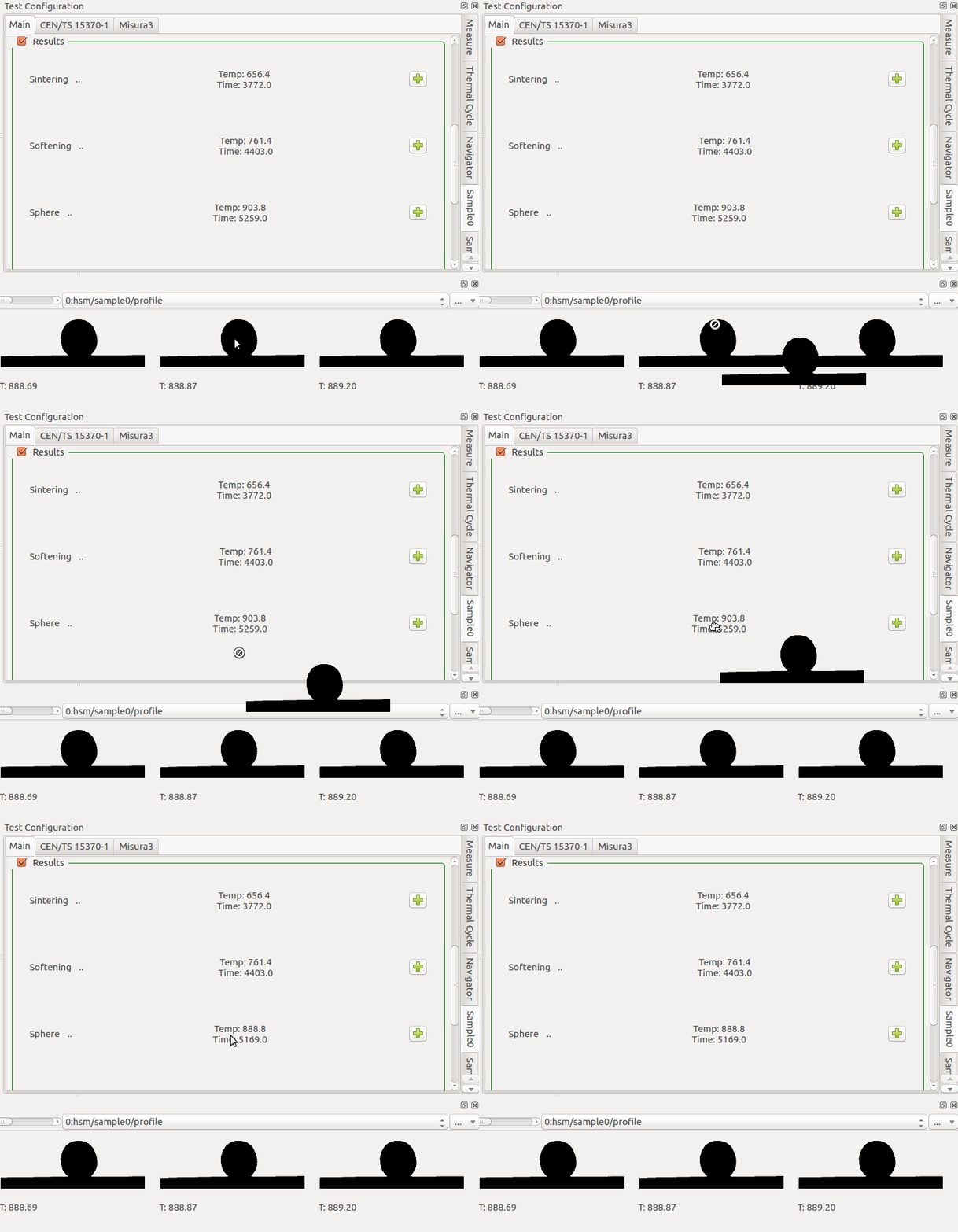
- Drag & drop the frame image onto the target point’s label.
In the following example, the Sphere point was changed from 908°C to 888°C:
Interacting with the Data Plot
As you have seen for Characteristic Points, the Navigator tree is the gate to the most important actions you can perform on the data plot.
In order to plot one more dataset (for example the height):
- Right-click on the dataset you wish to plot on the Navigator tree (
/hsm/sample0/h). - Select the Plot action from the context menu.
The same apply for removing a dataset and all its related objects from the plot. The Plot action will be checked if the curve is visible, unchecked if not visibile.
Mathematical manipulations: Smoothing
A frequently used feature is the Smoothing of a dataset. In order to smooth the volume, for example:
- Locate the Vol (
/hsm/sample0/Vol) element in the Navigator tree under Results tab. - Right-click and select Smoothing.
- A dialog will appear. Click Apply.
- A new temporary label in the dialog confirms the dataset was created. Click Close.
- The Navigator tree is updated. The Vol element now has a child: Smooth(48,Vol). This is the smoothed Vol dataset.
- Plot the smoothed dataset using its context menu.
The new dataset will be plotted over the old one, with the same color and just slight differences (mostly visible in the first 200s or 50°C). You can either un-plot the old one, or change the color of one of the two.
To change the color of the curve:
- Click on the curve on the Data Plot.
- Right-click again on the same spot. A context menu opens. Choose Formatting.
- Select the second tab, with a Line symbol.
- Change the color to something distinguishable (eg: red).
Creating a Report
Sample reports summarize the most meaningful data about a test run and a single sample behaviour in a printable page.
- Identify the Navigator tree element for the sample you are about to create a report for. E.g.:
/hsm/sample0. - Right-click on the element and select
Report. A new dialog opens: click Apply. - A temporary label Done appears. Click Close.
- Reports are rendered as new
pagesin the Data Plot. Right-click anywhere in the Data Plot and select Next page. - Wait some secons for the rendering of the report to complete.
- Reports are rendered as new
- The Data Plot displays the report.
- Right-click anywhere in the Data Plot and select the Export action.
- Select the location of the output PDF file.
The exported report is vector quality. Compare your result with Microscope Sample Report 1.pdf.
Creating a report listing all images
Listing all images, according to temperature and time steps, can be accomplished by the Export images action. It can be reached either:
- By right-clicking on the
sample0vertical tab title in the Test Configuration panel on the right. - From the context-menu of
sample0node in the Navigator (right-click on the node). - From the Storyboard, by right-clicking the slider or clicking on the … button on the extreme right.
- In this case, time/temperature stepping will be inherited from the current storyboard settings.
This action will output an HTML document listing all images, according to the selected starting/ending temperature and temperature/time stepping.
Compare your result with Microscope Sample Images 1.html.
Exporting to a Video
- Identify the Navigator tree element for the sample you are about to create a report for. E.g.:
/hsm/sample0. - Right-click on the element and select
Render video. - On Microsoft Windows™, a native dialog will open asking the desired output video encoding. Choose according to your supported formats.
- You can click Cancel anytime without loosing the partially rendered video.
Compare your result with Microscope Sample Video 1.avi.
Hint
Install Xvid MPEG4 video compression filter in order to get smaller video outputs.