Wizard Tutorial
This step-by-step guide will explain how to:
- Open and use the wizard built into Misura™ Flash,
- Navigate through the wizard’s different functionalities,
- Run model analysis on shots, segments, and samples.
From FlashLine to Misura™ Flash
Misura™ Flash needs to convert and compress a FlashLine test folder into a single HDF5 file in order to elaborate it.
- Open the Misura™ Browser by double-click on browser.exe.
- Locate the Data Sources sub-window, under the first Databases tab.
- Click on the Import button under the Recent files: column.
- Navigate to the
TestInformation.xmlfile, located in the root of your FlashLine test folder, and click Open. - The import process will require some minutes, depending on the speed of your computer, disk and network connection if the file is remote. The progress will be indicated by a dialog window containing a progress bar.
- After the import finishes, a pop-up dialog will ask to Start the Wizard or open the Default Plot. Select Start the Wizard for now.
Wizard: General Options
The Misura™ wizard will open to the General Options page, where different parameters for file can be set, such as:
- Click the drop-down menu next to Preferred Curve-Fitting Model and select the desired model for analysis of the test. Note: This is the only selection that is mandatory to set to move to the next step in the wizard.
- To set a Diffusivity Reference for the whole test, select the an option from the second drop down menu. This is step is optional. Note: Set individual reference values for each sample by clicking on the check box to expand the sample options, and then select a Diffusivity Reference.
- To set a System Geometry for the whole test, select an option from the third drop-down menu. This step is optional. Note: In some cases, |f| will automatically determine the system geometry and import it into Misura™. If that is the case, this option may be selected already, you can override value. Also, like Diffusivity Reference, you can set a differnt System Geometry for each sample.
At the bottom of the Wizard view are the controls for navigating through the Wizard. At this point, click Select Shot to move to the next section.
Wizard: Shot Selection
The orange arrows highlight the flow in selecting a shot to model:
- Select a sample from the rightmost box.
- Once the segment values appear in the middle box, select a temperature value.
- Select a shot from the final box.
- A preview of the shot will be shown in the middle window.
Click Modeling to move to the next section.
Wizard: Modeling
This section of the Wizard is for prototyping parameter values for the analysis of a shot. Below is a description of the three main components of this page of the Wizard:
- The shot on display:
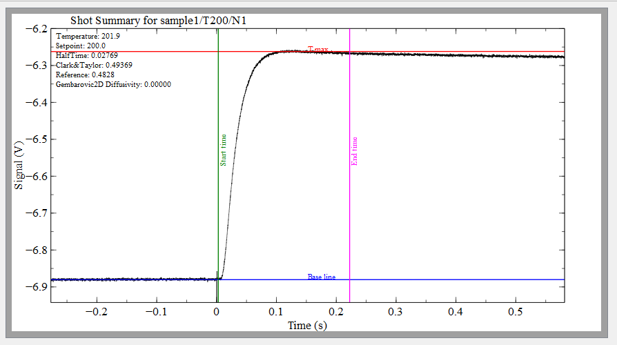
This is a normal shot plot with 4 colored lines on it, each representing differnt model parameters: - Start Time represents the Analysis start time parameter. - End Time represnts the Analysis end time parameter. - Tmax represents the Tmax parameter. - Base line represents the Baseline level parameter. You can click and drag each line to test different values.
- The parameter window:
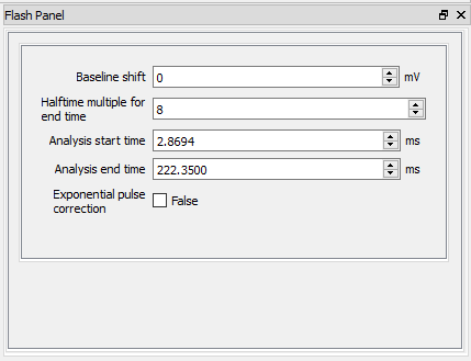
- This parameter window will initially show parameters that a user may commonly alter and test.
- The values in this window change a line in the shot plot gets clicked and dragged.
- If a value is changed in this window, the corresponding line in the shot plot will move to match the parameter value.
- To access all of the model parameters that a user can alter, click on the plot.
- The geometry diagram:
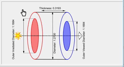
- This diagram is a representation of the sample and geometry.
- The labeled numbers match the values set in the sample geometry section of the parameter window.
- To view the Sample Geometry and Flash Geometry parameters in the parameter window, click on the diagram.
Before running a model, test out some of this functionality: #. In the parameter window, click the up-arrow on the value of Halftime multiple for endtime a couple times. #. Notice the line for End time move a short distance to the right. #. Now, select the End time line by clicking on it. #. Click and drag the line back left, roughly to where it began. #. The value for Halftime multiple for endtime will decrease to match the End time line. #. The same behavior will be observed for each line on the shot plot. #. Now click the geometry diagram. #. Notice that the parameter window now has the parameters for Sample Geometry and Flash Geometry*. #. Also, notice how the values for each parameter match up with the labled values in the diagram. #. Now click on an area of open space in the graph. #. Notice that the parameter window now contains all changeable parameters relevant to the model.
Once happy with the values for the model, click Run: Shot > to run the analysis.
Wizard: Shot Analysis
Once the model has finished running, it is time to analyze the results:
- The model plot is displayed in the wizard. The top half of the plot is the curve fit, and the bottom half is for the residuals.
- In the top left of the plot is the calculated diffusivity value for the model. Note: if a reference was set, then it will appear underneath the calculated diffusivity along with the percent difference between the two.
- At the top of the parameter window, there is a tab for results, if the user would like to see more information from the analysis.
- If the results are unfavorable, you can alter parameter values the same way as in the above section for Wiard: Modeling. Click Run: Shot > to run the model again.
- If happy with the results, you can run a recursion.
- To run a segment recursion, click Segment >.
- The pop-up provides a a list of all the parameter values set for the model incase you want to review them. Also, you can opt to skip running shots that were already analyzed.
- Click Ok in the pop-up to run the segment.
Once the segment completes, the wizard will display the segment sumary plot.
Wizard: Segment Analysis
- The segment plot is on display.
- In the top left corner of the plot is the table summary of the results.
- There is a red vertical line on the plot which can be dragged to any X coordinate to align the shots at that coordinate.
- Next, you can run a sample recursion by clicking Sample >, but before you do, check out the hints below.
Hint 1: To view a specific shot, right click on the button < Select shot and then left click on one of the drop down options. Hint 2: To run the segment again, you may alter parameters to how you want, then click Segment >.
Wizard: Sample Analysis
Once the sample recursion completes, the wizard will display the summary sample plot.
- View the sample plot.
- At the bottom left corner of the plot is the table summary of the results.
- Next, you can run a recursion on the whole test by clicking Test >, but before you do, check out the hints below.
Hint 1: To view a specific shot plot or segment plot, right click on the button < Select shot or < Segment and then left click on one of the drop down options. Hint 2: To run the sample again, you may alter parameters to how you want, then click Segment >.
Warning: Test recursion may take a while.
Wizard: Test Analysis
Once the test recursion completes, a sample test plot will be displayed.
Click the Save button to save your analysis progress to another version of the test file.
Click the Close Wizard button to exit the wizard view and operate misura from the default view.